Au - SiO2 - Au Multilayered Nanoparticle Project
Recently, the attention of some computational chemists has been turning to nanoparticle chemistry. In my lab, we are investigating how a multilayered nanoparticle will interact with light.

With the increase of abilities in computational chemistry, one can find vast amounts of information on his or her hard drive with minimal effort. Hours spent in the lab carefully designing experiments and producing substances for testing are reduced to a couple of scripts. That being said, handling the data from computational experiments can become cumbersome if the proper machinery isn’t in place. Thus, the aim of this project is to create a machine to handle data from the recent multilayered nanoparticle jobs.
The appropriate machine would be double edged: the first being the database itself, and the second would act as a post-processing application to interface with different users. The application would need to connect to the database, call upon different tables depending on what the user specifies, and display the relevant information. Here, I will show the creation of said database and the post-processing application.
Experimental Procedure
Independent Variables
Using the DDSCAT program on the University of Memphis’s HPC, the research group has run in total 78 different experiments. Each experiment had one or multiple of the following parameters modified:
- Au Core Size: the radius of the Au core in nm.
- SiO2 Layer Size: the width of the SiO2 layer in nm.
- Au Shell Size: the width of the Au outer layer in nm.
- Inner Layer/Outer Layer: identifies wether the measurements are taken at the surface of the core or the surface of the Au shell.
A table of all experimental conditions computed can be found at the end of the page. Each experiment computed results for both the inner layer and outer layer.
Dependent Variables
Each experiment returns multiple arrays of data. From the inner and outer layer, we collect data in the form of Qext, Qsca, Qabs, and E2 for a list of wavelengths (usually 400nm to 1000nm). These measurements are unitless.
Design
Analyzing $78\times4 = 312$ columns of data can be cumberson. However, I am enrolled an a database systems class. Therefore, in an effort to kill two birds with one stone, we will create a database of all the datapoints. This method can be tough to initialize, but once the ball is rolling, a simple query for any combination of experimental parameters will yeild the data set we wish to analyze with eaze.
Preprocessing
The raw data needs pre-processing after the experiment itself is finished. We begin by processing the raw data to be better fit into the mySQL database. The .txt files from the research group were extracted from the HPC, organized in folders by experiment, combined for both inner sphere and outer sphere measurements, and then combined completely into one master .txt file containing rows for wavelength ($\lambda$), Q${ext}$, Q${sca}$, Q$_{abs}$, E$^{2}$, and experimental conditions.
Finally, the master file was split into two files, one containing the results columns, and the other containing the experimental conditions. Both contain a column for the expID which is the foreign key for the results table referencing the conditions table where it is the primary key. In order for the .txt files to be added by command into the database, we translated the .txt information into .csv format. All pre-processing was done through multiple .py scripts.
SQL Schema
Now that we have two .csv files containing correctly formatted data, we initialize the database by creating two tables: Results and Conditions. The .csv files are then imported. Below is the schema for the database. After learning about database systems, the pre-processing procedure prepared the project’s data, so this portion of the project was trivial.
SQL Implimentation
Finally, we begin to interact with the data. The aim is to gather data from the database on the command of the user and graph the data. Ideally, this is a closed system in order to increase its user friendliness. Therefore, a .py script was developed for this purpose. However, since the database is hosted on my local machine, the database would need to be ported to some online network if I wanted to allow other users access.
The .py script asks the user for multiple pieces of information to locate the desired information. Below, I will walk through each step.
The first question asks the user for the amount of WHERE clauses they will want to add to the overall SQL statement. If a user wants only the data from jobs that had a coreSize of 5nm, they will enter in the indented lines (>). A list of all the conditional settings are given for reference.
How many WHERE clauses do you want to add?
> 1

0:	expID
1:	coreSize
2:	sio2Size
3:	shellSize
4:	outerBoolean

Please enter your WHERE clause (ex: "coreSize = 5"):
> coreSize = 5
After the script compiles an SQL command using this information, it asks the user what attributes he or she wants graphed.
How many series do you want to map?
> 1

0:	expID
1:	lambda
2:	qEXT
3:	qSCA
4:	qABS
5:	eSQU

Please select index of series:
> 3
Finally, all information has been provided, and the script will visualize the selected data using the ` Matplotlib} python package.
Evaluation / Analysis / Results
After development of the database and accompanying post-processing script, we are able to produce images of the spectra we ask for. Below is a sample spectra when the above code is executed.
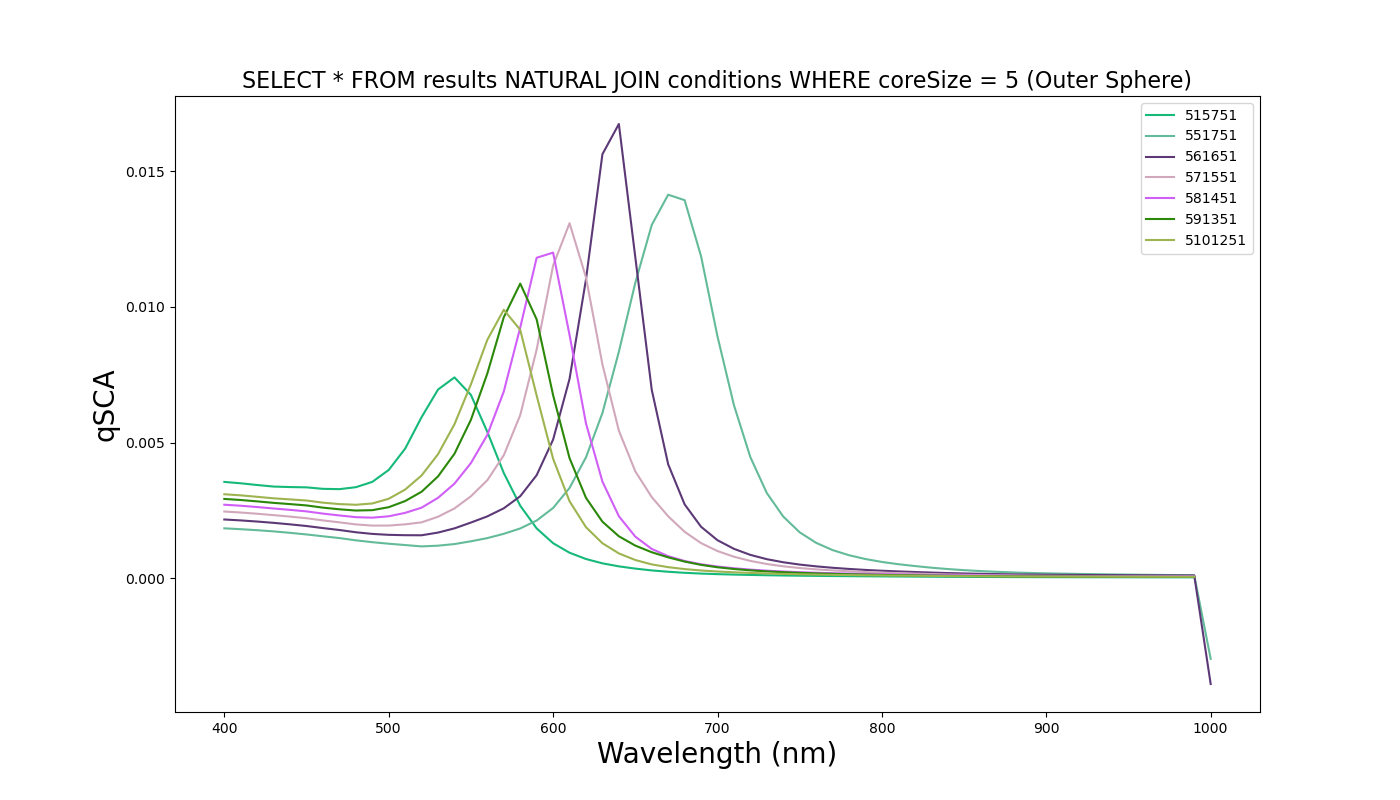
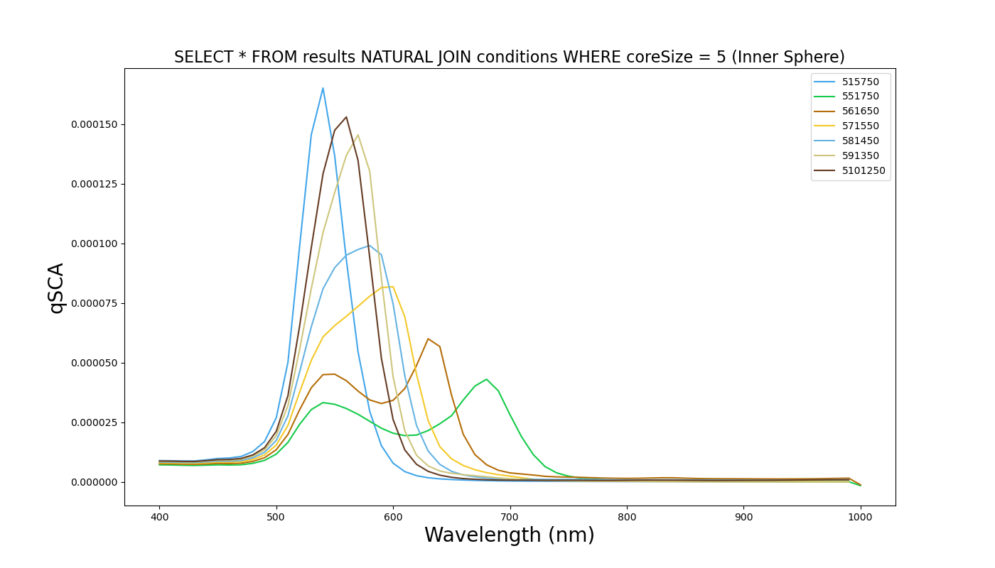
The script is capable of producing graphs on command of every combination of experiments and output parameters. Given the slew of .py scripts to pre-process the data, adding more experiments to the database is simple.
If this database were to grow to the point where storage was a concern, the extraction of experimental conditions into its own table reduces the hard drive size by reducing duplicate information.
Experiments Conducted
| Au Core Size | SiO2 Layer Size | Au Shell Size |
|---|---|---|
| 5nm | 5nm | 17.5nm |
| 5nm | 6nm | 16.5nm |
| 5nm | 7nm | 15.5nm |
| 5nm | 8nm | 14.5nm |
| 5nm | 9nm | 13.5nm |
| 5nm | 10nm | 12.5nm |
| 5nm | 15nm | 7.5nm |
| 10nm | 5nm | 15nm |
| 10nm | 6nm | 14nm |
| 10nm | 7nm | 13nm |
| 10nm | 8nm | 12nm |
| 10nm | 9nm | 11nm |
| 10nm | 10nm | 10nm |
| 10nm | 15nm | 5nm |
| 10nm | 17.5nm | 2.5nm |
| 15nm | 5nm | 12.5nm |
| 15nm | 6nm | 11.5nm |
| 15nm | 7nm | 10.5nm |
| 15nm | 8nm | 9.5nm |
| 15nm | 9nm | 8.5nm |
| 15nm | 10nm | 7.5nm |
| 15nm | 11nm | 6.5nm |
| 15nm | 12nm | 5.5nm |
| 15nm | 13nm | 4.5nm |
| 15nm | 14nm | 3.5nm |
| 15nm | 15nm | 2.5nm |
| 20nm | 10nm | 2.5nm |
| 20nm | 10nm | 7.5nm |
| 20nm | 10nm | 10nm |
| 20nm | 10nm | 12.5nm |
| 25nm | 3.5nm | 9nm |
| 25nm | 4.5nm | 8nm |
| 25nm | 5nm | 7.5nm |
| 25nm | 5.5nm | 7nm |
| 25nm | 6.5nm | 6nm |
| 25nm | 7.5nm | 5nm |
| 25nm | 8.5nm | 4nm |
| 25nm | 9.5nm | 3nm |
| 25nm | 10.5nm | 2nm |
Pre and Post Processing Files
- First Pre-Processing File (to be run on HPC)
- Second Pre-Processing File (to be run on local machine where all files have been gathered)
- SQL Database
- Post-Processing File